This hands-on post aimed at senior undergraduate and graduate students in CS illustrates the amplification trick due to Grover that is central to Quantum Search. Basic familiarity with python and linear algebra (tensor multiplication) is helpful to appreciate the trick and the construction of the quantum circuit. An understanding of Quantum Mechanics is not needed to understand and use Grover’s algorithm. The following beliefs are sufficient to appreciate the power of Quantum i) $n$ particle system keeps track of $N=2^n$ states in its belly, and ii) state changes can be accomplished efficiently by manipulating few particles (local changes) at a time.
The reflection
From now on, all vectors under consideration i) have either +ve or -ve entries and ii) the norm is 1. This reason for normalizing the vector to a vector with norm 1 is that such vectors represent the state of the quantum system with complex entries. Define the average of a vector as the sum of all the entries divided by the number of entries. The average of the entries in vector psi is the sum of the absolute values in the vector sum(psi)/N.
import math
import numpy as np

n = 3; N = 8 ;

psi =  np.array([+1, +1, +1, +1, +1, -1, +1, +1])
psi = 1/math.sqrt(N) * psi
print("psi: \n", psi)

avg = sum(psi)/N
print("average is : ", avg)
psi:
 [ 0.35355339  0.35355339  0.35355339  0.35355339  0.35355339 -0.35355339
  0.35355339  0.35355339]
average is :  0.2651650429449553
Grover’s trick reflects each entry in the vector around the mean of the vector. It is easy to visualize the reflection if we view each value $\theta$ as a vector with an angle $\theta$ from the origin to a point on the unit circle. The reflection operation reflects each entry around the average vector. The reflection operation can be defined as below. It can be verified that the result of the reflection is still a norm one vector.
import numpy as np
def reflect(vec, N):
    res = np.copy(vec)          #make a copy and return the result in res
    av = sum(vec)/N
    for i in range(N) :
        if (vec[i] <= av) :
            res[i] = av + (av - vec[i])
        else:
            res[i] = av - (vec[i] - av)
    return res

reflection = reflect(psi,8)  # the reflection
print(reflection)
print(np.dot(reflection, np.transpose(reflection))) # check for the norm.

# reflection = (2*sum(psi)/N)*np.ones(N) - psi
[0.1767767  0.1767767  0.1767767  0.1767767  0.1767767  0.88388348
 0.1767767  0.1767767 ]
0.9999999999999997
An examination of the code shows that the update to the vector is same in both the cases (each entry $a$ is replaced by $2*avg - a$). Therefore, reflection can be implemented as
reflection = (2*sum(psi)/N)*np.ones(N) - psi
The effect of this change is supposed to be two-fold i) the positive entries are reduced (and closer to zero) and ii) the negative entries become positive and farther away from 0. However, all the entries are now positive, which means we have lost information as which input $x$ was important. To restore the sign, we used the signed version of the function $F^{\pm}$ and query the state vector using the n particle quantum system. Construction of $F^{\pm}$ given $f$ is a fairly standard technique in Quantum Algorithms and will be explained separately in a future post. It is important to note that $F^{\pm}(reflect(psi))$ restores the signs on the reflected vector and we obtain
[+0.1767767 +0.1767767 +0.1767767 +0.1767767 +0.1767767 -0.88388348 +0.1767767 +0.1767767 ]. This new correctly signed version of the reflection becomes the next input, and the process repeats. One has to be careful to stop this iterative process while there is an improvement, as long as the average is positive. If the average is -ve then the improvement listed at the start of this paragraph is not guaranteed.
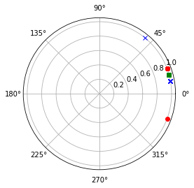
A visualization of the reflect operation is shown next.
The original vector has two different angles marked by a red ‘o’ in the plot below. The average angle is shown using a green square. The reflections are around the green square are marked using an x.
import numpy as np
import matplotlib.pyplot as plot

avg = sum(psi)/N

for theta in psi:
    plot.polar(theta, 1, 'ro')

plot.polar(avg, 1, 'gs')

reflection = (2*sum(psi)/N)*np.ones(N) - psi

for theta in reflection:
    plot.polar(theta, 1, 'bx')

plot.show()
Reflection as Matrix Multiplication
The reflect operation can also be described as matrix multiplication. Let $I, P$ be square matrices of order $N \times N.$ If $I$ is the identity matrix and each entry in $P$ is $1/N$ then $G= 2*P - I$ is the matrix that performs the reflection. Let’s verify this with the reflection vector computed earlier.
import numpy as np
import math

N = 8

G = -np.eye(N) + 2/N* np.ones((N,N))
print(G @ psi)  # @ is matrix multiply
[0.1767767  0.1767767  0.1767767  0.1767767  0.1767767  0.88388348
 0.1767767  0.1767767 ]
The matrix $G$ is symmetric and its own inverse. Moreover, $G$ can be described as a product of unitary matrices. If $H^N$ is the Hadamard matrix of order $N$ and $R$ a matrix with -1 in the first diagonal position, 1s on the rest main diagonal and 0 elsewhere.Then $G= - H^N R H^N.$ As illustrated next, the unitary operator $G$ can be implemented locally, that is the implementation uses polynomially many gates in the number of qubits.
from scipy.linalg import hadamard
R = np.eye(N)
R[0,0] = -1
H = 1/math.sqrt(N)*hadamard(8)
Reflect = - H @ R @ H
print(Reflect @ psi)
[0.1767767  0.1767767  0.1767767  0.1767767  0.1767767  0.88388348
 0.1767767  0.1767767 ]
It is Unitary: the Circuit
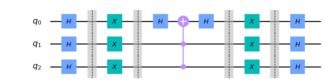
For the rest of this post, we assume basic familiarity with Quantum Circuits. You should be comfortable reading the output of quatum circuits at various points in time and might want to review Hadamard, X, Z, CCZ gates before proceeding with the rest. Let us just focus on the quantum circuit for $H R H$, where $H, R$ are defined as above. The circuit will have three qubits—the first operation on each qubit a Hadamard transform. The $R$ matrix acts on the first qubit, rest of the bits are unchanged. $R$ operation is implemented in three stages. In the first stage, $X$ gate is applied to all the qubits. In the second stage, $H$ gate is applied to qubit 0, then a CCZ gate is applied with target qubit 0, and the remaining two qubits are the control, and $H$ gate is reapplied to qubit 0. In the third stage, $X$ gate is applied again to all the qubits. The construction can be generalized for any number of qubits.
from qiskit import *

R = QuantumCircuit(3) # implement R matrix as a CCZ gate (in general C^nZ gate)
R.barrier()
R.x(0)
R.x(1)
R.x(2)
R.barrier()
R.h(0)
R.ccx(1,2,0)
R.h(0)
R.barrier()
R.x(0)
R.x(1)
R.x(2)
R.barrier()
R.draw('mpl')
Let’s also check the unitary transform of the $R$ circuit above to see if it indeed is the matrix we are expecting. The unitary simulator below does the job, and indeed $R$ circuit works as expected.
backend = Aer.get_backend('unitary_simulator')

job = execute(R, backend)
result = job.result()

print(result.get_unitary(R, decimals=3))
[[-1.+0.j -0.+0.j  0.+0.j  0.+0.j  0.+0.j  0.+0.j  0.+0.j  0.+0.j]
 [-0.-0.j  1.-0.j  0.+0.j  0.+0.j  0.+0.j  0.+0.j  0.+0.j  0.+0.j]
 [ 0.+0.j  0.+0.j  1.-0.j  0.+0.j  0.+0.j  0.+0.j  0.+0.j  0.+0.j]
 [ 0.+0.j  0.+0.j  0.+0.j  1.-0.j  0.+0.j  0.+0.j  0.+0.j  0.+0.j]
 [ 0.+0.j  0.+0.j  0.+0.j  0.+0.j  1.-0.j  0.+0.j  0.+0.j  0.+0.j]
 [ 0.+0.j  0.+0.j  0.+0.j  0.+0.j  0.+0.j  1.-0.j  0.+0.j  0.+0.j]
 [ 0.+0.j  0.+0.j  0.+0.j  0.+0.j  0.+0.j  0.+0.j  1.-0.j  0.+0.j]
 [ 0.+0.j  0.+0.j  0.+0.j  0.+0.j  0.+0.j  0.+0.j  0.+0.j  1.-0.j]]
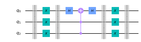
The circuit to perform the reflection can now be constructed. The first and the last stage in the circuit below are the Hadamard gates applied to each qubit, and the middle part is the $R$ circuit.
n=3
N = 2^n

reflect = QuantumCircuit(3)

reflect.h(0)
reflect.h(1)
reflect.h(2)

reflect = reflect + R + reflect

reflect.draw('mpl')
Once again we use the unitary simulator to check is the unitary is the same as the matrix Reflect above. Convince yourself that the unitary is the same.
backend = Aer.get_backend('unitary_simulator')

job = execute(reflect, backend)
result = job.result()

print(result.get_unitary(reflect, decimals=3))
[[ 0.75-0.j -0.25+0.j -0.25+0.j -0.25+0.j -0.25+0.j -0.25+0.j -0.25+0.j
  -0.25+0.j]
 [-0.25+0.j  0.75-0.j -0.25+0.j -0.25+0.j -0.25+0.j -0.25+0.j -0.25+0.j
  -0.25+0.j]
 [-0.25+0.j -0.25+0.j  0.75-0.j -0.25+0.j -0.25+0.j -0.25+0.j -0.25+0.j
  -0.25+0.j]
 [-0.25+0.j -0.25+0.j -0.25+0.j  0.75-0.j -0.25+0.j -0.25+0.j -0.25+0.j
  -0.25+0.j]
 [-0.25+0.j -0.25+0.j -0.25+0.j -0.25+0.j  0.75-0.j -0.25+0.j -0.25+0.j
  -0.25+0.j]
 [-0.25+0.j -0.25+0.j -0.25+0.j -0.25+0.j -0.25+0.j  0.75-0.j -0.25+0.j
  -0.25+0.j]
 [-0.25+0.j -0.25+0.j -0.25+0.j -0.25+0.j -0.25+0.j -0.25+0.j  0.75-0.j
  -0.25+0.j]
 [-0.25+0.j -0.25+0.j -0.25+0.j -0.25+0.j -0.25+0.j -0.25+0.j -0.25+0.j
   0.75-0.j]]
The circuits for the initial step of data preparation and the signed query operator $Q_F^{\pm}$ will be examined in a later post. Grover’s method [4] is known to be optimal and has been simplified and works for function where the number of solutions ($|{x : f(x)=1}|$) is not known in advance [1]. Grover’s method has also been artfully applied to finding the minimum [2] and for counting [3].
Exercises:
Do the following to execute this code on an IBM Quantum machine.
- prepare and load the
psivector into the machine, - add measurements at the end of the circuit, and
- change the
Aer.get_backend('unitary_simulator')with one of the IBM Q machines.
Further Reading:
[1] Boyer M, Brassard G, Hoyer P, Tapp A. Tight bounds on quantum searching. Fortschritte der Physik: Progress of Physics. 1998 Jun;46(4‐5):493-505.
[2] Durr, Christoph, and Peter Hoyer. “A quantum algorithm for finding the minimum.” arXiv preprint quant-ph/9607014 (1996).
[3] Brassard, Gilles, Peter Hoyer, and Alain Tapp. “Quantum counting.” International Colloquium on Automata, Languages, and Programming. Springer, Berlin, Heidelberg, 1998.
[4] Grover, Lov K. “A fast quantum mechanical algorithm for database search.” Proceedings of the twenty-eighth annual ACM symposium on Theory of computing. 1996.