Here's a quick tutorial on using some features of Maple in support of your
courses. More details can be had by using Maple's online help functions, and
by consulting Maple manuals. This is by no means a comprehensive account of
these aspects of Maple, and programming in Maple is not addressed at all.
There are a number of ways Maple can be invoked. If you are at a workstation,
the full graphical front end to Maple can be brought up by invoking Maple from
a terminal window by typing xmaple or maple -x at the
terminal window's prompt machine_name$. Bringing Maple up this way uses the
Java runtime environment which can be very slow. For a faster, lighter Maple
session, bring up graphical Maple environment by typing the command
maple -cw at the prompt in the command
window. The interface is different, but it retains all the functionality of
the Java version.
If you are connecting from a different site (for example, your home PC) to
telnet.cs.uleth.ca, or don't need or want the graphical front-end to
Maple, you can invoke Maple simply by typing maple at the prompt.
To quit from a graphical session (invoked as xmaple or
maple -x or maple -cw), go to the "File" menu and select the option "Exit". Wait a
few seconds before logging out, as it will take a few seconds for Maple to
clean up after itself before returning the prompt in the terminal window from
which you started Maple.
If you are running a text-only session (invoked by maple), simply
type quit at the Maple prompt. The command quit is one of the
few
exceptions to Maple's syntax of requiring either a semicolon or colon following
a command. Maple will then exit, print a brief summary of statistics concerning
your session, and return your machine's prompt.
Maple provides some very handy functions for dealing with linear algebra.
Below is a Maple session illustrating some of the functionality of the
linear algebra tools. Commentary is interspersed with the session.
Maple also inserts blank lines to ease readability. These have been removed
from the sample session.
nefarius$ maple
    |\^/|     Maple V Release 5 (University of Lethbridge)
._|\|   |/|_. Copyright (c) 1981-1997 by Waterloo Maple Inc. All rights
 \  MAPLE  /  reserved. Maple and Maple V are registered trademarks of
 <____ ____>  Waterloo Maple Inc.
      |       Type ? for help.
> with(linalg);
Warning, new definition for norm
Warning, new definition for trace
[BlockDiagonal, GramSchmidt, JordanBlock, LUdecomp, QRdecomp, Wronskian,
    addcol, addrow, adj, adjoint, angle, augment, backsub, band, basis, bezout,
    blockmatrix, charmat, charpoly, cholesky, col, coldim, colspace, colspan,
    companion, concat, cond, copyinto, crossprod, curl, definite, delcols,
    delrows, det, diag, diverge, dotprod, eigenvals, eigenvalues, eigenvectors,
    eigenvects, entermatrix, equal, exponential, extend, ffgausselim,
    fibonacci, forwardsub, frobenius, gausselim, gaussjord, geneqns, genmatrix,
    grad, hadamard, hermite, hessian, hilbert, htranspose, ihermite, indexfunc,
    innerprod, intbasis, inverse, ismith, issimilar, iszero, jacobian, jordan,
    kernel, laplacian, leastsqrs, linsolve, matadd, matrix, minor, minpoly,
    mulcol, mulrow, multiply, norm, normalize, nullspace, orthog, permanent,
    pivot, potential, randmatrix, randvector, rank, ratform, row, rowdim,
    rowspace, rowspan, rref, scalarmul, singularvals, smith, stackmatrix,
    submatrix, subvector, sumbasis, swapcol, swaprow, sylvester, toeplitz,
    trace, transpose, vandermonde, vecpotent, vectdim, vector, wronskian]
If you didn't want the long list of components in the linear algebra package
appearing, then instead of typing with(linalg); with its trailing
semi-colon, you could just type with(linalg): (i.e., use a trailing
colon rather than a semicolon to suppress output).
To get help on any of these functions, type ?function-name at the ">"
prompt. No trailing semicolon is required.
> ?cond
linalg[cond] - condition number of a matrix

Calling Sequence:
     cond(A)
     cond(A, normname)

Parameters:
     A        - a square matrix
     normname - (optional) matrix norm, must be one of: 1, 2, 'infinity', or
'frobenius'.

Description:
- The function cond computes the ``standard'' matrix condition number, defined
  as norm(A) * norm(inverse(A)). The matrix norm is the default employed by
  the linalg[norm] function, namely the infinity norm (maximum row sum).

- More generally, cond(A, normname) computes norm(A, normname) *
  norm(inverse(A), normname). This is the same measure, but using the
  specified norm instead of the infinity norm.

- The command with(linalg,cond) allows the use of the abbreviated form of this
  command.
In the newest release of Maple, a separate window opens displaying the help
file information for this.
Manipulating matrices is very straightforward in Maple.
> A:=matrix(3,3,[4,1,0,1,4,1,0,1,4]);
                                   [4    1    0]
                                   [           ]
                              A := [1    4    1]
                                   [           ]
                                   [0    1    4]
> B := [2,1,3];
                                B := [2, 1, 3]
> multiply(A,B);
                                  [9, 9, 13]
Maple is smart enought to know that the vector B must be interpreted as
a column vector in this instance.
> X0 := [1,1,1];
                                X0 := [1, 1, 1]
> L:=matrix(3,3,[0,0,0,1,0,0,0,1,0]);
                                   [0    0    0]
                                   [           ]
                              L := [1    0    0]
                                   [           ]
                                   [0    1    0]
> Dg:=matrix(3,3,[4,0,0,0,4,0,0,0,4]);
                                    [4    0    0]
                                    [           ]
                              Dg := [0    4    0]
                                    [           ]
                                    [0    0    4]
> U:=matrix(3,3,[0,1,0,0,0,1,0,0,0]);
                                   [0    1    0]
                                   [           ]
                              U := [0    0    1]
                                   [           ]
                                   [0    0    0]
> evalm(A);
                                 [4    1    0]
                                 [           ]
                                 [1    4    1]
                                 [           ]
                                 [0    1    4]
> evalm(L+Dg+U);
                                 [4    1    0]
                                 [           ]
                                 [1    4    1]
                                 [           ]
                                 [0    1    4]
Doing matrix inverses? Notice this:
> evalm(1/Dg);
                              [1/4     0      0 ]
                              [                 ]
                              [ 0     1/4     0 ]
                              [                 ]
                              [ 0      0     1/4]
> evalm(X0);
                                   [1, 1, 1]
> X1 := evalm((1/Dg)*(B - (L+U)*X0));
bytes used=1001056, alloc=720764, time=0.33
                            X1 := [1/4, -1/4, 1/2]
> X2 := evalm((1/Dg)*(B - (L+U)*X1));
                                  [            13]
                            X2 := [9/16, 1/16, --]
                                  [            16]
> X3 := evalm((1/Dg)*(B - (L+U)*X2));
                                    [31  -3  47]
                              X3 := [--, --, --]
                                    [64  32  64]
> X4 := evalm((1/Dg)*(B - (L+U)*X3));
                                   [67   -7   99 ]
                             X4 := [---, ---, ---]
                                   [128  128  128]
> X5 := evalm((1/Dg)*(B - (L+U)*X4));
                                   [263  -19  391]
                             X5 := [---, ---, ---]
                                   [512  256  512]
> evalf(263/512);
                                  .5136718750
> evalf(-19/256);
                                 -.07421875000
> evalf(391/512);
                                  .7636718750
Maple will perform exact arithmetic. To render a fraction as a decimal
(or decimal approximation), the evalf function is used, as illustrated
above.
Maple can easily cope with row-reductions of matrices. With the matrix A
above, the reduced row-echelon form is obtainable with the rref
function:
> rref(A);
                                 [1    0    0]
                                 [           ]
                                 [0    1    0]
                                 [           ]
                                 [0    0    1]
Routine differentiation can be easily managed in Maple. For example, suppose
we have calculated that
yp =
e2x((7/5)cos x - (1/5)sin x)
is a solution to the differential equation
y'' - y' + 2y =
e2x(cos x - 3sin x),
but want to check our
solution. We can easily verify this using Maple's build-in ability to differentiate expressions.
First, let us assign a label f to our expression
for yp,
> f:=exp(2*x)*((7/5)*cos(x)-(1/5)*sin(x));
                    f := exp(2 x) (7/5 cos(x) - 1/5 sin(x))
We need first and second derivatives of f, so
use the diff operator to compute them and save the results in
df and ddf, respectively:
> df:=diff(f,x);
df :=

    2 exp(2 x) (7/5 cos(x) - 1/5 sin(x)) + exp(2 x) (-7/5 sin(x) - 1/5 cos(x))

> ddf:=diff(df,x);
ddf := 4 exp(2 x) (7/5 cos(x) - 1/5 sin(x))

     + 4 exp(2 x) (-7/5 sin(x) - 1/5 cos(x))

     + exp(2 x) (-7/5 cos(x) + 1/5 sin(x))
With the first and second derivatives of yp
in hand, we compute the left hand side of our differential equation:
> ddf-2*df +2*f;
2 exp(2 x) (7/5 cos(x) - 1/5 sin(x)) + 2 exp(2 x) (-7/5 sin(x) - 1/5 cos(x))

     + exp(2 x) (-7/5 cos(x) + 1/5 sin(x))
There are some cancellations that can be performed here,
but we can get Maple to do that for us with the simplify command:
> simplify(%);
                         exp(2 x) (cos(x) - 3 sin(x))

>
The percent symbol is Maple's shorthand for the output
of the previous command.
Achieving this result validates our answer.
Plotting is best done in the X/Window invocation of Maple (start with
maple -x or xmaple or maple -cw).
> plot(x * (x-1) * (x+1), x=-5..5);
A simple graph of this cubic polynomial will appear as output. Notice the
syntax of the plot command: the first argument is an expression in
an independent variable, followed by the range of the variable. By re-issuing
the plot command with different intervals, you can "zoom in" or "zoom
out" on the graph. Try the previous command with the intervals
x=-1.5..1.5 and x=-10..10 to see the effect for yourself.
The command ?plot will provide you with additional information about
options to the plot command. Also, if you issue the plot
command in a Maple text window session, Maple will fashion a reasonable
facsimile of the graph using keyboard characters (an example of this follows).
A helpful timesaver in both the text-only and X/Windows forms of Maple is
command recall. By using the "up arrow" key, you can recall a previous command
and just edit that instead of re-typing the command. In the X/Windows form,
the "up arrow" key will move the cursor up through previous lines in your
session.
You can define functions in Maple as well for easy subsequent use. For
example,
> f := x -> (x^2 + 3*x)/(x^4 + x + 1);
defines the rational function f(x) = (x2 + 3x)/(x4
+ x + 1), and subsequent computations with this rational functional can be
done using f(x):
> f := x -> (x^2 + 3*x)/(x^4 + x + 1);
                                         2
                                        x  + 3 x
                             f := x -> ----------
                                        4
                                       x  + x + 1

> f(1);
                                      4/3

> evalf(f(1));
                                  1.333333333

> plot(f(x), x=-5..5);

                                       +    AAAA
                                       +  AA   AAA
                                      1+  A      AAA
                                       + A         AA
                                       +AA           AAAA
                                       +A                AAAAAAA
  ******-4************--2--+--+--+--+--*--+--+--+--+--2--+--+--+*****4*******
                      AAAAA           0*
                          AAA         A+
                            AA        A+
                             A       A +
                              A      -1+
                              A     AA +
                               A    A  +
                               A    A  +
                               A    A-2+
                                A  AA  +
                                A  A   +
                                A  A   +
                                 AAA   +
                                 AA  -3+
In an X/Windows session, the graph would be nicely drawn. You might find it
interesting to try plotting functions that have singularities, to see how Maple
copes with problem functions.
Maple can also handle functions that are piecewise defined. The appropriate
command to use is piecewise, and the syntax is
piecewise( 1st condition, 1st function, 2nd condition,
2nd function, etc., otherwise function).
So, if we wanted a function definition that was sin(x) for x < 1,
and then 2*x+1 for 1 <= x < 2, and then 1-x^3, we could code it up as
g:=piecewise(x < 1, sin(x), 1 <= x and x< 2, 2*x+1, 1-x^3);
Try graphing g using the plot command to see for yourself.
Try using the plotting option discont=true to rid your graph of
artifacts of the plotting process.
For the denominator in our rational function f, you might try to
see if it vanishes anywhere. Maple has built-in facilities for root-finding.
To search for an exact solution to an equation p(x) = 0, use
solve(). If this does not produce a solution in closed form, you can
look for a solution numerically with fsolve:
> solve(x^4 + x + 1 = 0, x);
bytes used=1014064, alloc=851812, time=0.28
                                      4
                             RootOf(_Z  + _Z + 1)
This is Maple's way of stating that it was unable to obtain an exact solution.
We can continue by searching for a numerical solution:
> fsolve(x^4 + x + 1 = 0);
In this case, no result is returned, so numerical methods failed to produce
a solution to the equation. A slight modification of this problem will show you
what to expect to see when solutions do exist:
> solve(x^4 + x + 1 = 4);
                                      4
                             RootOf(_Z  + _Z - 3)
> fsolve(x^4 + x + 1 = 4);
                           -1.452626879, 1.164035140
Maple can also plot implicitly defined functions. Issue the with(plots)
command to load an enhanced graphics library:
> with(plots);
[animate, animate3d, animatecurve, changecoords, complexplot, complexplot3d,
    conformal, contourplot, contourplot3d, coordplot, coordplot3d,
    cylinderplot, densityplot, display, display3d, fieldplot, fieldplot3d,
    gradplot, gradplot3d, implicitplot, implicitplot3d, inequal, listcontplot,
    listcontplot3d, listdensityplot, listplot, listplot3d, loglogplot, logplot,
    matrixplot, odeplot, pareto, pointplot, pointplot3d, polarplot,
    polygonplot, polygonplot3d, polyhedra_supported, polyhedraplot, replot,
    rootlocus, semilogplot, setoptions, setoptions3d, spacecurve,
    sparsematrixplot, sphereplot, surfdata, textplot, textplot3d, tubeplot]
You should spend some time browsing this rich set of tools. For now, suppose
we want a plot of the ellipse x2 + 2(y - 1)2 = 4.
The implicitplot function is the appropriate tool to use for this task:
> implicitplot(x^2+2*(y-1)^2 = 4, x=-4..4, y=-4..4);
Maple obligingly supplies a graph. implicitplot can be very
helpful when drawing the isoclines for a differential equation.
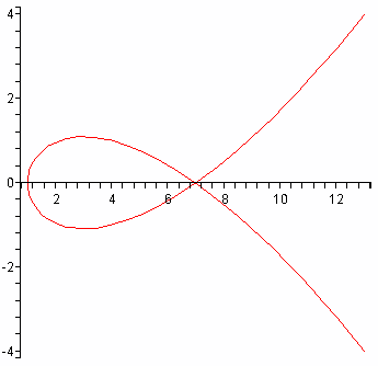 Plotting of parametrically defined curves can also be done. For example,
to plot the plane curve x = 1 + 3t2,
y = t3 -2t, first ensure you have the graphical
front end of Maple running (by invoking either xmaple or
maple -x or maple -cw from the Unix command line), and then define the functions
f and g by the Maple commands
> f:=t->1+3*t^2;
> g:=t->t^3-2*t;
Maple responds by pretty-printing these function definitions. To plot the
curves with t ranging from, say, -2 to 2, issue the command
>plot([f(t),g(t),t=-2..2]);
Maple produces the figure at right.
Plotting polar curves produces no great difficulties. To plot a curve
expressing r as a function of an angle, first define r as a
function of the angle, and then plot the Cartesian equations as above.
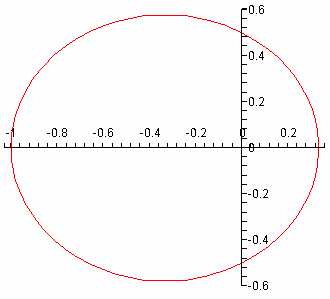 For example, to plot the ellipse given by r = 1/(2 + cos(theta)),
we define r by r:=theta->1/(2+cos(theta)) to which Maple responds
by pretty-printing the function definition, and then issue the plot command
> plot([r(theta)*cos(theta), r(theta)*sin(theta),
> theta=0..2*Pi], scaling=constrained);
Notice that Pi is a built-in constant for Maple. The corresponding
figure produced will indeed be that of an ellipse, though if you omit the option
scaling=constrained from the plot command, what you'll see will be more
like a circle due to Maple's default action of scaling axes to fill out the
command window.
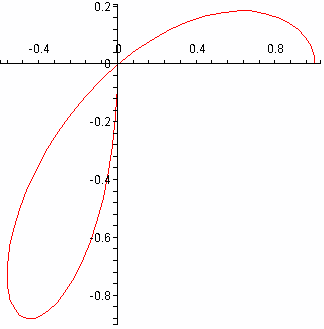 A more interesting polar curve is a three-leaved rose, given by r =
cos(3*theta). If plotted as for the previous example with, say,
r1:=theta->cos(3*theta) used to define r as a function of theta,
then the full curve is traced out, of course, with theta varying from 0 to
2*Pi. You can analyse the curve using smaller intervals for theta, though.
Using the interval from 0 to Pi will trace out the full curve, and if you
restrict theta further, say to [0, Pi/2], using the command
plot([r1(theta)*cos(theta), r1(theta)*sin(theta), theta=0..Pi/2]), the
figure at the right results.
To plot parametric curves in space requires the use of the plots
package, so make sure you have loaded the package into your active Maple session
by typing with(plots): into the command window in Maple if you haven't
already done so.
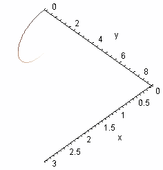 Let us plot the parametric space curve x = t, y =
t2, z = t3 with t ranging over
the interval [0, 3].
We could define functions for each of the coordinates x, y and
z as we did for our first parametric curve in the plane, but this one is
simple enough to do directly. Issue the command
spacecurve([t,t^2,t^3], t=0..3, axes=frame,labels=[x,y,z]);
in the Maple command window. Maple produces the figure at the right, which
sadly is not very helpful.
The options in the spacecurve command provide axes and labels for
the coordinate axes and can be modified or omitted as you see fit.
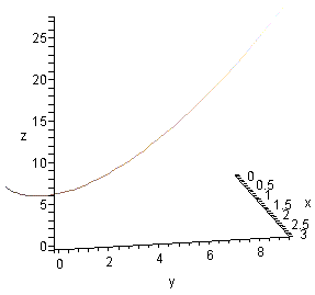 Notice that when you
move the mouse pointer over the figure, the pointer changes into a curved arrow.
If you click and hold the right mouse button while the curved pointer is visible,
as the pointer moves the figure itself will rotate. This allows you to view
the curve from a number of different points, and gives you a better sense of the
three-dimensional character of the plot than would otherwise be the case for a
fixed, static, image.
The image at the right is one of the many possible
views that result when rotating the image, and the labelling of the coordinate
axes is a great help in determining the view you are getting of the curve.
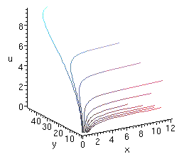
Multiple curves can be plotted on the same graph. To illustrate this, we take
as an example the first order PDE used to illustrate the method of characteristics
found in the text by Carrier and Pearson: the PDE is
x2ux + uuy = 1
with initial data u = 0 along the line x + y = 1 for
x > 0. The curve along which the data are given is a non-characteristic
curve, and the characteristics themselves are curves issuing from points along
the non-characteristic curve that evolve according to the first order DEs
dx/dt = x2, dy/dt = u, and du/dt = 1,
for which we have
x = s/(1 - st), y = (1/2)t2 + 1 - s, u = t,
where s is used to parametrise the non-characeteristic curve x =
s, y = 1 - s, with s > 0.
To plot several of these characteristic curves (starting from the non-characteristic
curve at t = 0), we define them first by
x:=(t,s) -> s/(1-s*t);
y:=(t,s) -> t^2/2+1-s;
y:=(t,s) -> t;
which Maple dutifully pretty-prints. The plotting is accomplished by
spacecurve({[x(t,0.1),y(t,0.1),u(t,0.1), t=0..9.6],
[x(t,0.15),y(t,0.15),u(t,0.15), t=0..6.55],
[x(t,0.2),y(t,0.2),u(t,0.2), t=0..4.9],
[x(t,0.3),y(t,0.3),u(t,0.3), t=0..3.25],
[x(t,0.4),y(t,0.4),u(t,0.4), t=0..2.4],
[x(t,0.5),y(t,0.5),u(t,0.5), t=0..1.85],
[x(t,0.6),y(t,0.6),u(t,0.6), t=0..1.55],
[x(t,0.7),y(t,0.7),u(t,0.7), t=0..1.33],
[x(t,0.8),y(t,0.8),u(t,0.8), t=0..1.15],
[x(t,0.9),y(t,0.9),u(t,0.9), t=0..1.02]},
axes=frame,labels=[x,y,u]);
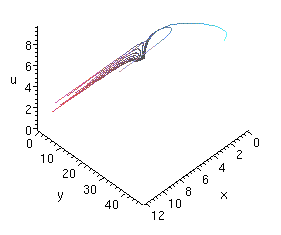
which results in the graph (three views are shown)
If you haven't yet done so, start up Maple with the graphical front-end by
either typing xmaple or maple -x or maple -cw into a command window, and
load the graphics library by typing, in the Maple command window, the statement
> with(plots):
We'll explore some possibilities for plotting surfaces in this section.
Remember that Maple commands must always be terminated by semicolons, even if
the examples shown here don't always reflect this fact.
First, here's how to plot a simple surface given as a function of two
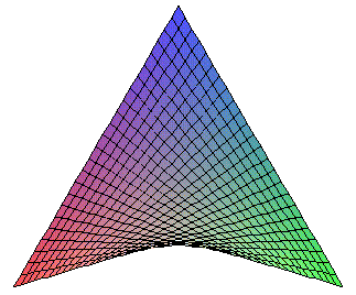
variables. We'll use the example of g(x,y) = xy,
which has a saddle surface (hyperbolic paraboloid) as its graph. To start, define
the function g by issuing the command
> g:=(x,y)->x*y;
 Maple will respond by nicely printing your function definition for you. To
generate a plot requires the specification of ranges of x and y
values. Type
> plot3d(g(x,y),x=-3..3,y=-3..3);
into the command window to generate the graph of g with x and
y each ranging over the interval [-3,3]. This will produce the plot
seen at the right. If you move your mouse pointer over the graph in the Maple
window, the cursor will change into a curved arrow, and if you click and hold
the left mouse button and slowly move the curved cursor around, you'll see
the plotted image rotate. By playing with the rotations this way, you'll be
able to get a sense of how the surface fits into space.
This plot of the saddle surface was done using simple defaults in the plot3d
command. To gain some idea of the range of options possible with the plot3d
command, type the command ?plot3d,options into the Maple command
window. A new window (the help window) will pop open with a description of the
plot3d command, along with examples and options. Close the help window and type
the command
> plot3d(g(x,y),x=-5..5,y=-5..5,style=patchnogrid);
 into the command window and Maple will produce a new saddle surface plot,
without grid lines. The plot at the right is what you should expect (here, the
figure has been rotated to more clearly show the saddle). plot3d has a
sizeable number of options, and it is well worth the time to experiment with
different options and parameter values.
The plots library of functions can also do plotting of surfaces
defined implicitly. For example, to plot the plane with equation 4x -
2y + z = 8, you could issue the command
> implicitplot3d(4*x - 2*y + z = 8, x=-3..3,y=-3..3,z=-3..3);
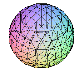
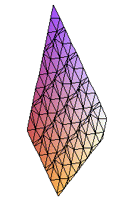 and Maple would respond by generating a plot of that portion of the plane
found in the rectangular box [-3,3]×[-3,3]×[-3,3]. With a little more
sophistication, multiple plots of surfaces can be incorporated into the same
graphic. For example, to simultaneously plot a plane and sphere in the same
figure, issue the commands
> plane:=4*x-2*y+z=8;
> sphere:=x^2+y^2+z^2=9;
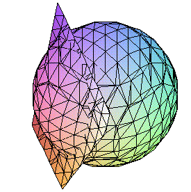 This symbolically labels the equations defining each of a plane and a sphere
for subsequent, easier reference. If you issue
implicitplot3d(plane, x=-3..3, y=-3..3, z=-3..3) and
implicitplot3d(sphere, x=-3..3, y=-3..3, z=-3..3)
commands, then you will generate separate plots of the plane and the sphere, as
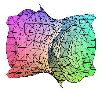
illustrated above at right. To incorporate both surfaces in the same plot,
though, issue the single command
implicitplot3d({plane,sphere}, x=-3..3, y=-3..3, z=-3..3)
and Maple will produce the figure at right (this time presented full size from
the Maple session used to generate these graphics).
 Notice that the different surfaces being simultaneously plotted in the one
implicitplot3d are enclosed in curly braces {...} and separated by
commas. The same idea can be used without resorting to individually labelling
each constituent equation. For example, if we wished to plot the three level
surfaces f(x,y,z) = -1,
f(x,y,z) = 0 and
f(x,y,z) = 1
for the function f(x,y,z) = x2
- y2 + z2, then first define the function
in the command window by typing f:=(x,y,z)->x^2-y^2+z^2 and then issue
the command implicitplot3d({f(x,y,z)=-1, f(x,y,z)=0, f(x,y,z)=1}, x=-1.2..1.2,
y=-1.2..1.2, z=-1.2..1.2) to produce the striking figure at the right (or above,
depending on your browser and the width you've selected for the window).
As before, if you use the mouse to rotate the surfaces, additional insight can
be had into how these surfaces are placed in space (in this case, a hyperboloid
of one sheet wraps around a cone through the origin which in turn has each nappe
containing one component of an hyperboloid of two sheets).
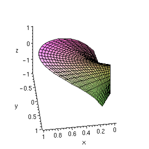
Maple can also plot parametrised surfaces. For example, for the surface
with chart (or patch)
x(u,v) = (u cos v,
u sin v, u + log cos v)
where v is restricted to the open interval from -Pi/2 to Pi/2, we can
get an image of this surface (for u restricted to (0,1) and v
restricted to (-1.4, 1.4)) by issuing the plot command
plot3d([u*cos(v),u*sin(v),u+log(cos(v))], u=0..1, v=-1.4..1.4,
axes=frame,labels=[x,y,z])
.
The result is shown below.
Happy plotting!
The plots library contains other specialised tools for plotting.
Here, we just mention the use of the gradient plotting function gradplot.
If you have not done so, load the plots library into Maple by typing
the command with(plots); into the command window. Then try the command
gradplot(x^3*y^2/(x^2+y^2),x=-2..2,y=-2..2);
Maple responds by generating a plot of the gradient vector field associated
with the function (in this case, the function is
x3y2/(x2
+ y2)):
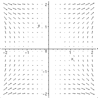
Some additional insight into this vector field can be seen by plotting the
function and viewing it from several angles. Use the command
plot3d(x^3*y^2/(x^2+y^2),x=-2..2,y=-2..2,axes=BOXED);
and view it from several different angles to try to reconcile the gradient field
plot with the surface plot you see.
Maple has a library of functions for use in manipulating differential
equations, DEtools. Load this now:
> with(DEtools);
[DEnormal, DEplot, DEplot3d, DEplot_polygon, DFactor, Dchangevar, GCRD, LCLM,
    PDEchangecoords, RiemannPsols, abelsol, adjoint, autonomous, bernoullisol,
    buildsol, buildsym, canoni, chinisol, clairautsol, constcoeffsols,
    convertAlg, convertsys, dalembertsol, de2diffop, dfieldplot, diffop2de,
    eigenring, endomorphism_charpoly, equinv, eta_k, eulersols, exactsol,
    expsols, exterior_power, formal_sol, gen_exp, generate_ic, genhomosol,
    hamilton_eqs, indicialeq, infgen, integrate_sols, intfactor, kovacicsols,
    leftdivision, liesol, line_int, linearsol, matrixDE, matrix_riccati,
    moser_reduce, mult, newton_polygon, odeadvisor, odepde, parametricsol,
    phaseportrait, poincare, polysols, ratsols, reduceOrder, regular_parts,
    regularsp, riccati_system, riccatisol, rightdivision, separablesol,
    super_reduce, symgen, symmetric_power, symmetric_product, symtest,
    transinv, translate, untranslate, varparam, zoom]
The command DEplot is especially useful in the early part of the
study of differential equations.
For example, to build a direction field for the DE dy/dx = x2 - y2
over a grid in the x-direction from -4 to 4, and in the y-direction
from -3 to 3, enter:
> de := D(y)(x) = x^2 - y(x)^2;
                                           2       2
                          de := D(y)(x) = x  - y(x)

> DEplot(de,y(x),x=-4..4, y=-3..3, arrows=THIN,scaling=constrained);
The first line of input is the statement of the differential equation in
Maple terms, with y's dependence on x explicitly stated. The
derivative is expressed as D(y)(x). The entire DE has been labelled
as de so that we don't have to re-type in subsequent commands.
The DEplot command is shown with a number of options (use
?DEplot to see more), and with an X/Windows Maple session running,
you will obtain an attractive plot of the direction field for this DE.
A slight change to this DEplot command will also graph solutions
to initial value problems (IVPs). Instead of the DEplot we used above,
issue the command:
> DEplot(de,y(x),x=-4..4, {[y(-2)=0]}, y=-3..3);
Maple will produce a direction field plot again over the same grid in the
xy-plane, but now with a curve superimposed on the grid which shows
the solution to the IVP with initial data y(-2) = 0.
DEplot can be used with coupled systems of differential equations in
much the same fashion. Suppose we want to analyse the system (a competition
model)
(d/dt)N1 = N1((1 - N1/5)
- N2/10)
(d/dt)N2 = N2((1 - N2/5)
- N1/10)
The system can be described by the Maple definition
> de2 := [diff(N1(t),t)=N1*((1-N1/5) - N2/10), diff(N2(t),t)=N2*((1-N2/5) - N1/10)];
To plot the direction field with solution curves issuing, at t = 0,
from points (N1, N1) = (2,1), (6,1), (6,6)
and (1,7), we would use DEplot in the form
> DEplot(de2, [N1(t),N2(t)], t=0..5,
>	{[N1(0)=2,N2(0)=1],[N1(0)=6,N2(0)=1],
>	[N1(0)=6,N2(0)=6],[N1(0)=1,N2(0)=7]},
>	N1=0..8, N2=0..8);
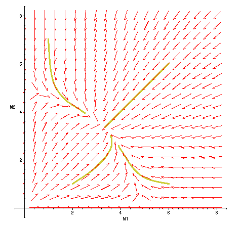 Maple then obligingly produces the figure displayed at the right (it will squawk,
however, about variable names).
From the
illustration produced, we can clearly see the equilibrium point "attracting"
solutions issuing from different parts of the
N1N2-plane. The equilibrium point, by the
way, is readily found to be (10/3, 10/3), and the lines in the first quadrant
for which either (d/dt)N1 = 0 or
(d/dt)N2 = 0 are easily determined as
N2 = 10 - 2N1
and
N2 = 5 - N1/2,
respectively.
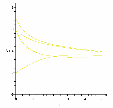 If we alter our last DEplot command to
> DEplot(de2, [N1(t),N2(t)], t=0..5,
> {[N1(0)=2,N2(0)=1],[N1(0)=6,N2(0)=1],
> [N1(0)=6,N2(0)=6],[N1(0)=7,N2(0)=1]},
> N1=0..8, N2=0..8,scene=[t,N1]);
(i.e., we add the parameter "scene=[t,N1]" at the end of the command)
then instead of producing the direction field plot we had obtained before,
we now get plots of N1(t), one for each initial value in the
solutions presented in the direction field plot.
Maple can also exactly solve limited classes of DEs (and produce numerical
solutions, if desired). For example, to solve the second order DE y'' - y'
- 2y = x, you could issue the commands:
> eq := (D@@2)(y)(x)-D(y)(x)-2*y(x)=x;

              (2)
      eq := (D   )(y)(x) - D(y)(x) - 2 y(x) = x

> dsolve(eq, y(x));
bytes used=5215952, alloc=2358864, time=2.53
                y(x) = 1/4 - 1/2 x + _C1 exp(2 x) + _C2 exp(-x)
The dsolve command is the relevant tool here. In the definition of
the DE (which here is labelled "eq"), you can see how to express a second-order
derivative. In the solution Maple was able to furnish, you'll notice the
expression of two arbitrary constants _C1 and _C2. This is
what we would expect to happen in the solution of a second order equation. For
dsolve output in solving a first-order equation, we would anticipate
the presence of a single arbitrary constant in the general solution.
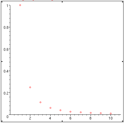
Maple can be a useful tool for exploring properties of sequences and series.
To illustrate, let us look at a p-series with p = 2. Define the sequence
{1/n2} by
a := n -> n^(-2);
Maple responds by pretty-printing the definition of the sequence.
To see the first ten terms of this sequence, use the sequence command seq:
seq(a(n),n=1..10);
Maple will respond by computing the sequence elements an
for n ranging from 1 to 10, and pretty-printing the result as fractions.
Plotting is a little more involved. First, we generate a list of the
sequence elements we want to plot:
sequencepoints := [seq([n,a(n)], n=1..10)];
Of course, you could call the list of ordered pairs (i, ai)
something other than sequencepoints. Maple responds by generating
the desired list of ordered pairs. To plot an
versus i, issue the command plot:
plot(sequencepoints, 0..11, 0..1, style=point, symbol=circle);
The result is a graph like that below.

If you consult Maple's Help on the plot command, you will see other options
available to you. The first range in the plot command, 0..11, indicates the
range of the ordinate to be used in the graph. The second range, 0..1, gives
the range of the abscissa to be used in building the graph. Try using the same
command, this time without specifying the second range. Try the command again,
this time specifying the option symbol=cross in the plot command.
Maple can also do limits. We know that 1/n2 goes to 0
as n tends to infinity; so does Maple:
Limit(a(n), n=infinity);
Maple responds by pretty-printing the limit. To get a value, next type
value(%);
The percent sign is Maple shorthand for the output of the previous command. In
this case, you should see Maple correctly answer "0" for the value of the limit.
To sum elements of a sequence, type
Sum(a(n), n=1..10);
Maple pretty-prints the sum and to see the value of this partial sum, issue
the command
value(%);
Maple responds with the exact value of the sum, expressed as a fraction. To
obtain a decimal approximation of this fraction, next issue the command
evalf(%);
This tells Maple to use the machine's floating point arithmetic to compute the
fraction, calculator style. Occasionally, Maple is also able to sum an infinite
series. For the sum of the full p-series with p = 2, try the command
Sum(a(n), n=1..infinity);
Maple again pretty-prints the series, and to see if Maple can calculate a
value for the sum of the series, try
value(%);
In this case, Maple can evaluate the sum of the series, and responds with a
pretty-printed exact value. To obtain a decimal approximation to this, again
issue the command
evalf(%);
If Maple cannot evaluate a series, it won't and will let you know.
Sometimes, Maple can determine if a series diverges, too. For example, define
the terms in the harmonic series by
h := n -> 1/n;
As usual, Maple pretty-prints the function definition. Then try summing the
harmonic series:
Sum(h(n), n=1..infinity);
Maple pretty-prints the series, but now if you issue the command
value(%),
Maple responds by printing the infinity symbol to indicate that the series
diverges to infinity.
What does Maple do if a series' divergence or convergence can't be determined?
Try this exercise: define the sequence of alternating 1s and (-1)s by
d := n -> (-1)^n;
Then trying summing it:
Sum(d(n), n=0..infinity);
As expected, the series is pretty-printed. What results now if you issue the
command value(%)?
You can use the Limit command to aid you in applying convergence tests.
For example, to apply the ratio test to the series of terms given by
b := n -> 2^n/(2*n)!;
try using the Limit function to compute the limit of the ratio of consecutive
terms in the sequence:
Limit(b(n+1)/b(n), n=infinity);
followed by value(%).
Last update: November 19, 2014.
© Copyright 2005-2014 David Kaminski.
 Plotting of parametrically defined curves can also be done. For example,
to plot the plane curve x = 1 + 3t2,
y = t3 -2t, first ensure you have the graphical
front end of Maple running (by invoking either xmaple or
maple -x or maple -cw from the Unix command line), and then define the functions
f and g by the Maple commands
 For example, to plot the ellipse given by r = 1/(2 + cos(theta)),
we define r by r:=theta->1/(2+cos(theta)) to which Maple responds
by pretty-printing the function definition, and then issue the plot command
 A more interesting polar curve is a three-leaved rose, given by r =
cos(3*theta). If plotted as for the previous example with, say,
r1:=theta->cos(3*theta) used to define r as a function of theta,
then the full curve is traced out, of course, with theta varying from 0 to
2*Pi. You can analyse the curve using smaller intervals for theta, though.
Using the interval from 0 to Pi will trace out the full curve, and if you
restrict theta further, say to [0, Pi/2], using the command
plot([r1(theta)*cos(theta), r1(theta)*sin(theta), theta=0..Pi/2]), the
figure at the right results.
 Let us plot the parametric space curve x = t, y =
t2, z = t3 with t ranging over
the interval [0, 3].
 Notice that when you
move the mouse pointer over the figure, the pointer changes into a curved arrow.
If you click and hold the right mouse button while the curved pointer is visible,
as the pointer moves the figure itself will rotate. This allows you to view
the curve from a number of different points, and gives you a better sense of the
three-dimensional character of the plot than would otherwise be the case for a
fixed, static, image.

 Maple will respond by nicely printing your function definition for you. To
generate a plot requires the specification of ranges of x and y
values. Type
 into the command window and Maple will produce a new saddle surface plot,
without grid lines. The plot at the right is what you should expect (here, the
figure has been rotated to more clearly show the saddle). plot3d has a
sizeable number of options, and it is well worth the time to experiment with
different options and parameter values.
 and Maple would respond by generating a plot of that portion of the plane
found in the rectangular box [-3,3]×[-3,3]×[-3,3]. With a little more
sophistication, multiple plots of surfaces can be incorporated into the same
graphic. For example, to simultaneously plot a plane and sphere in the same
figure, issue the commands
 This symbolically labels the equations defining each of a plane and a sphere
for subsequent, easier reference. If you issue
implicitplot3d(plane, x=-3..3, y=-3..3, z=-3..3) and
implicitplot3d(sphere, x=-3..3, y=-3..3, z=-3..3)
commands, then you will generate separate plots of the plane and the sphere, as
illustrated above at right. To incorporate both surfaces in the same plot,
though, issue the single command
implicitplot3d({plane,sphere}, x=-3..3, y=-3..3, z=-3..3)
and Maple will produce the figure at right (this time presented full size from
the Maple session used to generate these graphics).
 Notice that the different surfaces being simultaneously plotted in the one
implicitplot3d are enclosed in curly braces {...} and separated by
commas. The same idea can be used without resorting to individually labelling
each constituent equation. For example, if we wished to plot the three level
surfaces f(x,y,z) = -1,
f(x,y,z) = 0 and
f(x,y,z) = 1
for the function f(x,y,z) = x2
- y2 + z2, then first define the function
in the command window by typing f:=(x,y,z)->x^2-y^2+z^2 and then issue
the command implicitplot3d({f(x,y,z)=-1, f(x,y,z)=0, f(x,y,z)=1}, x=-1.2..1.2,
y=-1.2..1.2, z=-1.2..1.2) to produce the striking figure at the right (or above,
depending on your browser and the width you've selected for the window).
As before, if you use the mouse to rotate the surfaces, additional insight can
be had into how these surfaces are placed in space (in this case, a hyperboloid
of one sheet wraps around a cone through the origin which in turn has each nappe
containing one component of an hyperboloid of two sheets).

 Maple then obligingly produces the figure displayed at the right (it will squawk,
however, about variable names).
 If we alter our last DEplot command to
