This post is a follow-on to the post on the reflection trick in quantum computing. The recipe that we will learn hands-on in this post is again a viral trick that is used all over the place in quantum algorithms that rely on the query model of Boolean functions. The method will also give an alternate way to implement the operator $R$ in $HRH$ in the reflection part of Grover’s algorithm.
In the query model, boolean functions are used as a blackbox, $f$ on input $x$ returns $f(x)$, no other information (structural or otherwise) is available for the boolean function $f$. Usually, input to $f$ is a binary string and the output is $0,1$ (false/true). As usual $f$ has $n$ inputs, $1$ output, and the truth table for $f$ has size $N=2^n$. In the quantum setting, we need a quantum anlog of $f$ called $Q_f^{\pm}$ with two properties: + $Q_f^{\pm}(x) = +1,$ if $f(x) = 0$ and $Q_f^{\pm}(x) = -1$, otherwise + $Q_f^{\pm}$ has an efficient quantum circuit.
Assume that a $f$ has a classical implementation that is efficient (using poly($n$) constant fan-in gates) then $Q_f^{\pm}$ can be created using a standard recipe. In this post, we learn the method using an example. We will also query the circuit for the unitary operator (using unitary_simulator). We will test for the intended behaviour of the circuit on the on classical (pure), and quantum (superposition) states using the unitary. The simulation is purely illustrative as even for moderately sized circuits the unitary is exponential sized.
Boolean Function $f$
The example is chosen to demonstrate an alternate circuit for the $R$ operator (in $HRH$, see the post on reflection). We will work with the OR-3 function of three inputs. For $f=(a \vee b \vee c)$, we will take a classical circuit and construct the quantum circuit $Q_f^{\pm}$. We will assume basic familiarity with python, no specialized knowledge about quantum computing is needed to learn this useful trick of computing signed representations. The intended audience here is undergraduate and graduate students in CS, so read on.
The truth table for $f$ is below. True/False values for $a,b,c$ are denoted using $0/1$. The values for $a,b,c$ in each row can be read as a binary number, the corresponding number in decimal is in the first column. The output of the function $f (Q_f^{\pm})$ is in the second last (last) column. Our goal is to obtain a circuit for $Q_f^{\pm}$ given a circuit for $f$. We will build $Q_f^{\pm}$ in two stages. In the first stage, we build $Q_f$, which is simply the Quantum circuit for computing $f$ (with outputs 0/1). In the second stage, we modify the circuit for $Q_f$ ever so slightly to obtain the circuit for $Q_f^{\pm}.$
| index | $a$ | $b$ | $c$ | $f$ | $Q_f^{\pm}$ |
|---|---|---|---|---|---|
| 0 | 0 | 0 | 0 | F | +1 |
| 1 | 0 | 0 | 1 | T | -1 |
| 2 | 0 | 1 | 0 | T | -1 |
| 3 | 0 | 1 | 1 | T | -1 |
| 4 | 1 | 0 | 0 | T | -1 |
| 4 | 1 | 0 | 0 | T | -1 |
| 5 | 1 | 0 | 1 | T | -1 |
| 6 | 1 | 1 | 0 | T | -1 |
| 7 | 1 | 1 | 1 | T | -1 |
$f$ can be implemented using a tree of OR-gates (2-input and 1-output). This holds in general; one needs $n-1$ OR gates to achieve OR of $n$ bits. There is a bottleneck, however, OR gate is not one of the basic gates in Quantum Circuits. To get around this, we use i) the CCX gate (also known as the Toffoli gate) and the X gate to implement OR. See the paper by Feynman titled “Quantum Mechanical Computer” for details (link at the end).
OR-2 Gate
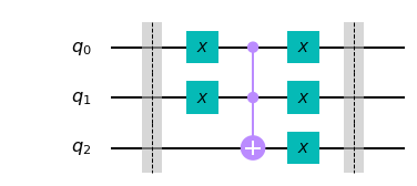
CCX gate three inputs (three outputs) two of which are control, and the third is the target. If both the controls are $1$, then the target bit is flipped by the CCX gate. A vector of length 8 describes the state of 3 bits. The action of the CCX gate can be modelled as an 8x8 matrix. The parallelism of the 3-particle quantum system guarantees that the next state is efficiently obtainable (not observable). If $x, y$ are the controls and $x$ the target then the output bits of CCX gate are $x,y, (x \wedge y) \oplus z$. If we set the target bit $z$ to $0$, then the output of the CCX gate is $x \wedge y$. Noting that, $a \vee b = \neg ( \neg a \wedge \neg b)$, following circuit implements an OR gate. The inputs $a,b$ have to be loaded appropriately before the call to the circuit. The first two output qubits ($q_0, q_1$) are the inputs supplied to the circuit, and the last qubit ($q_2$) is $q_0 \vee q_1$. For the math to work out nicely, the circuit should be reversible, i.e., one should be able to recover the input from the output, hence the two X gates on $q_0, q_1$ in the end.
from qiskit import *


ckt = QuantumCircuit(3) #global ckt
ckt.barrier()

def OR(a,b, c) : # a, b are controls and c is target (result)
    ckt.x(a)
    ckt.x(b)
    ckt.ccx(a,b,c) # c, c, target
    ckt.x(a)       # revert a
    ckt.x(b)       # revert b
    ckt.x(c)

# inputs a,b are provided to qubits q0, q1
# q2 is ancillary qubits needed for CCX

OR(0,1,2)         # q2 = q0 v q1 = a v b
ckt.barrier()
ckt.draw('mpl')
Let’s check the behaviour of the OR gate above. The inputs to the gate above are written as $q_2q_1q_0$. The classical data to the gate above are $000, 001, 010, 011.$ The table shows each index of the input and the index of the output (into the truth table vector). Make sure that you understand the correspondence between the binary strings and the index entry. This mode of representation is critical to the reasoning and understanding (see Quantum Algorithms via Linear Algebra by Lipton and Regan)
| Input ($q_2 q_1 q_0$) | Input Index | Output | Output Index |
|---|---|---|---|
| 000 | 0 | 000 | 0 |
| 001 | 1 | 101 | 5 |
| 010 | 2 | 110 | 6 |
| 011 | 3 | 111 | 7 |
The unitary corresponding to the matrix above is shown below. Let’s mulitply the unitary with the vectors $0=[0 0 0 0 0 0 0 0], 1=[1 0 0 0 0 0 0 0], 2=[1 1 0 0 0 0 0 0], 4=[0 0 1 0 0 0 0 0].$ The result of performing the multiplication is as expected. The circuit above implements the OR gate in a reversible manner. The 3 particle system manipulates indiviual particles (poly($n$)-gates in general) and the net result is equivalent to a matrix multiplication (of order $N\times N$), of course the particle system does not perform matrix multiplication. Note that the unitary is a permutation matrix.
import numpy as np

backend = Aer.get_backend('unitary_simulator')

job = execute(ckt, backend)
result = job.result()

Op = result.get_unitary(ckt, decimals=0)
print(Op.real)

print("Verfiying the Circuit")

print(Op.real @ np.array([1,0,0,0,0,0,0,0])) # input 0
print(Op.real @ np.array([0,1,0,0,0,0,0,0])) # input 1
print(Op.real @ np.array([0,0,1,0,0,0,0,0])) # input 2
print(Op.real @ np.array([0,0,0,1,0,0,0,0])) # input 3
[[1. 0. 0. 0. 0. 0. 0. 0.]
 [0. 0. 0. 0. 0. 1. 0. 0.]
 [0. 0. 0. 0. 0. 0. 1. 0.]
 [0. 0. 0. 0. 0. 0. 0. 1.]
 [0. 0. 0. 0. 1. 0. 0. 0.]
 [0. 1. 0. 0. 0. 0. 0. 0.]
 [0. 0. 1. 0. 0. 0. 0. 0.]
 [0. 0. 0. 1. 0. 0. 0. 0.]]
Verfiying the Circuit
[1. 0. 0. 0. 0. 0. 0. 0.]
[0. 0. 0. 0. 0. 1. 0. 0.]
[0. 0. 0. 0. 0. 0. 1. 0.]
[0. 0. 0. 0. 0. 0. 0. 1.]
$Q_f$ for OR-n Gate
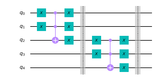
We need an extra qubit (called an ancillary qubit) to implement an OR of two inputs. So for each OR gate, we need an extra qubit. The general construction is below (try changing the value of $n$). The circuit for $n=3$ below implements $a \vee b \vee c$ using two extra qubits. The construction below uses poly($n$)-qubits ($2n-1$) to implement an OR of $n$ bits. Minimizing the number of ancillae needed to implement a classical circuit is an important optimization problem in the design of quantum circuits.
Once again remember to correctly load inputs $a,b,c$ in qubits $q_0, q_1, q_3$ respectively. The output is available in $q_4.$ The input qubits $q_0, q_1, q_3, q_5, \ldots $ all have two $X$ gate; therefore at the end output is the same as the input on these qubits. The ancilla $q_2, q_4$ have intermediate results $q_2 = q_0 \vee q_1, q_4 = q_2 \vee q_3$ which can be discarded at the end of the computation.
# Q_f
# General construction q0, q1, q3, q5, q7, ... data
# ancillary qubits are q2,  q4, ..q_{2n-2}
# result is in q_{2(n-1)}

n = 3
ckt = QuantumCircuit(2*n-1)

OR(0,1,2)
ckt.barrier()
for i in range(1,n-1):
    OR(2*i, 2*i+1, 2*i+2)
    ckt.barrier()

ckt.draw('mpl')
Once again let’s check the behaviour of the OR-3 using the unitary. The ancilla is always $0$ if the inputs $q_0 q_1 q_3$ are $000$ then for input $00000$ the output should be $00000$. The table below shows the classical inputs and corresponding outputs. The index of the non-zero entry (1) in the basis vector is shown under the index column.
| $q_4 q_3 q_2 q_1 q_0$ | Input Index | Output | Output Index |
|---|---|---|---|
| 00000 | 0 | 00000 | 0 |
| 00001 | 1 | 10101 | 21 |
| 00010 | 2 | 10110 | 22 |
| 00011 | 3 | 10111 | 23 |
| 01000 | 8 | 11000 | 24 |
| 01001 | 9 | 11101 | 29 |
| 01010 | 10 | 11110 | 30 |
| 01011 | 11 | 11111 | 31 |
As shown below, the outputs are as expected on the inputs in the table above.
#import numpy  as np

backend = Aer.get_backend('unitary_simulator')

job = execute(ckt, backend)
result = job.result()

Op = result.get_unitary(ckt, decimals=0)
print(Op.real)

print("Verfiying the OR-3 Circuit")

inputs = [0,1,2,3,8,9,10,11] # inputs

for x in inputs :
    inp = np.zeros(32)
    inp[x] =1
    print(np.where(Op.real @ inp == 1)[0]) # print the index
[[1. 0. 0. ... 0. 0. 0.]
 [0. 0. 0. ... 0. 0. 0.]
 [0. 0. 0. ... 0. 0. 0.]
 ...
 [0. 0. 0. ... 0. 0. 0.]
 [0. 0. 0. ... 0. 0. 0.]
 [0. 0. 0. ... 0. 0. 0.]]
Verfiying the OR-3 Circuit
[0]
[21]
[22]
[23]
[24]
[29]
[30]
[31]
Final Step: $Q_f^{\pm}$
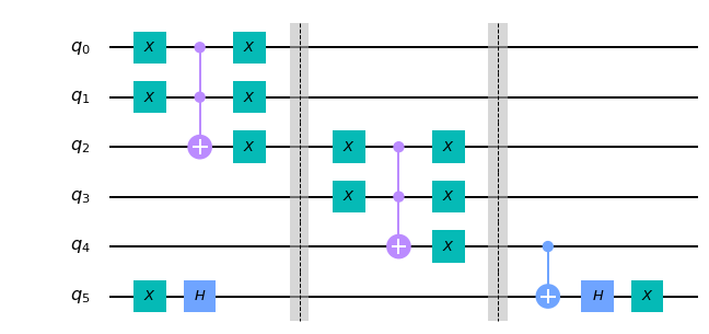
So far we have constructed a quantum circuit $Q_f$ given a classical function $f$. Next and the final step in this trick is to convert the output of $Q_f$ to $+1, -1$ (from $1,0$). For this a little familiarity with Dirac’s braket notation is needed. You may skip the rest of this paragraph on the first reading. This requires another ancilla, $q_5$ for our example. We modify the circuit for $Q_f$ such that $q_4 = q_5 \oplus Q_f(x)$ on input $x$. Suppose, $q_5$ is in state $1/\sqrt{2}(\mid{0} \rangle) - \mid{1} \rangle).$ Ignoring the normalizing constant, the state is $$\mid{x} \rangle) \otimes(\mid{0} \rangle - \mid{1} \rangle)$$ $$\mid{x~0} \rangle - \mid{x~1} \rangle$$ Application of $Q_f$ results in $$Q_f\mid{x~0} \rangle - Q_f\mid{x~1} \rangle $$ If $Q_f(x) = 0$ then the state is $$\mid{x~0} \rangle - \mid{x~1} \rangle = (-1)^{f(x)} (\mid{x} \rangle\otimes (\mid{0} \rangle - \mid{1} \rangle)$$ else ($Q_f(x) = 1$), the state is $$\mid{x~1} \rangle - \mid{x~0} \rangle = (-1)^{f(x)} (\mid{x} \rangle\otimes (\mid{0} \rangle - \mid{1} \rangle).$$ The previous two states are obtained through CX gate applied to $q_4$ with $q_5$ as the control. Thus we have $+1, -1$ instead to $0,1$. The question that remains is how to put $q_5$ in the desired state. Applying an $X$ gate, sets $q_5$ to $\mid{1} \rangle$ and $H \mid{1} \rangle$ is the desired state. The last step is to invert the $XH$ operations on $q_5$. This step reverts $q_5$ to $0$ and simplifies the bookkeeping, and we know where to expect the results.
In general, we need an extra qubit (numbered $2n-1$ below). We apply $XH$ gates to the last qubit and a CX gate to the output (penultimate qubit) with the last qubit as the control. Finally, we reverse the operations on the last qubit. The signed output for classical input $x$ to $f$ is in the penultimate qubit in the implementation below.
# Q_f^{\pm} (Signed Circuit)
# General construction q0, q1, q3, q5, q7, ... data
# ancillary qubits are q2,  q4, ..q_{2n-2}
# result is in q_{2(n-1)}
# last qubit is for b exor f(x)

n = 3
ckt = QuantumCircuit(2*n) # 2n-1 orginal

ckt.x(2*n-1)               # switch last qubit to 1
ckt.h(2*n-1)               # new state |0> - |1>

OR(0,1,2)
ckt.barrier()
for i in range(1,n-1):
    OR(2*i, 2*i+1, 2*i+2)
    ckt.barrier()

ckt.cx(2*n-2, 2*n-1) # q_4 = q_5 exor Q_f(x)
ckt.h(2*n-1)
ckt.x(2*n-1)         # reverse the XH so we know where the output is
ckt.draw('mpl')
The final step is the verification for which we use the table for $Q_f$. The output for $00 \ldots 0$ is $+1$ . For all other inputs, the output is $-1$, and this is as expected in the table above. You can uncomment the last few lines and check the output for any supervision as well. At this point you should have a fairly good understanding of Grover’s Quantum algorithm for searching unordered data.
If you have persevered so far, you might as well try the exercises. Feel free to drop an email in case there are any questions. Enjoy!
import math

backend = Aer.get_backend('unitary_simulator')

job = execute(ckt, backend)
result = job.result()

Op = result.get_unitary(ckt, decimals=0)
print(Op.real)

print("Verfiying the OR-3 Circuit")

inputs = [0,1,2,3,8,9,10,11] # inputs

for x in inputs :
    inp = np.zeros(64) # 6 qubits now
    inp[x] =1
    print("input x :", x, "output +1 at idx", np.where(Op.real @ inp == 1)[0]) # print the index

for x in inputs :
    inp = np.zeros(64) # 6 qubits now
    inp[x] =1
    print("input x :", x, "output -1 at idx", np.where(Op.real @ inp == -1)[0]) # print the index

# Let's check 1/sqrt(N)*ones(8)
#inp = np.zeros(64) # 6 qubits now
#for x in inputs :
#    inp[x] =1/math.sqrt(8)

#print ("Verifying uniform superposition")
#print("input x :", x, "output -1 at idx", np.where(Op.real @ inp == +1)[0]) # print the index
[[1. 0. 0. ... 0. 0. 0.]
 [0. 0. 0. ... 0. 0. 0.]
 [0. 0. 0. ... 0. 0. 0.]
 ...
 [0. 0. 0. ... 0. 0. 0.]
 [0. 0. 0. ... 0. 0. 0.]
 [0. 0. 0. ... 0. 0. 0.]]
Verfiying the OR-3 Circuit
input x : 0 output +1 at idx [0]
input x : 1 output +1 at idx []
input x : 2 output +1 at idx []
input x : 3 output +1 at idx []
input x : 8 output +1 at idx []
input x : 9 output +1 at idx []
input x : 10 output +1 at idx []
input x : 11 output +1 at idx []
input x : 0 output -1 at idx []
input x : 1 output -1 at idx [21]
input x : 2 output -1 at idx [22]
input x : 3 output -1 at idx [23]
input x : 8 output -1 at idx [24]
input x : 9 output -1 at idx [29]
input x : 10 output -1 at idx [30]
input x : 11 output -1 at idx [31]
Exercises
Operator $R$ in Grover’s amplification trick can be implement by $f0 = \neg f$ which is 1 on input $000 \ldots 0$, and $0$ else where. Build a poly($n$)-sized quantum circuit for computing $Q_{f0}^{\pm}.$
Build a poly($n$) sized quantum circuit for computing $Q_{EVEN}^{\pm}$ where $EVEN$ returns true if the number of $1s$ in the input is even, $0$ otherwise. Input is $n$-bits.
Add i) inputs, ii) measures, and iii) an appropriate
backendto the code above to execute the circuits above on an IBM Quantum machine.
Further Reading